Introduction to Programming and Scientific Applications (Spring 2020)
Final project
The goal of the final project is to do some concrete Python implementation and documenting it in a short report. The project can be done in groups with 1-3 students. There are three deliverables for the final project that should be handed in:
- Python code. Either plain Python 3 code in one or more .py files, or Python 3 code embedded into a Jupyter file.
- A report - maximum 4 pages. The front page must contain the information listed below (the front page does not count towards the page count).
- Visualization of data. E.g. matplotlib output. The plots should be included in an appendix to the report, that does not count towards the page count, or alternatively embedded in a Jupyter file.
Evaluation of handin
The project deliverables will be scored according to the following rubric:
| Deliverable | Not present 0% |
Many major shortcomings 25% |
Some major weaknesses 50% |
Minor weaknesses 75% |
Solid 100% |
|---|---|---|---|---|---|
| Code 50% |
No code, or code where no part computes the required | Some elementary parts of the code work, but significant parts do not work | Most essential parts of the code work, but the code does not completely solve the problem addressed | Overall good code, but space for improvement, e.g. missing documentation, code could be made clearer | Complete code, well structured, good use of modules, clear variable names, good documentation, PEP8 compliant |
| Visualization 25% |
No visualization | Very few or very unclear visualizations | Some visualizations illustrating basic idea | Overall good visualization but some details could have been more clear | Clear visualizations documenting the problem being solved and supporting the conclusions drawn |
| Report 25% |
No report | Very unpolished report, missing structure, no clear conclusions, major misunderstandings | The basic ideas are described but details are missing | Overall good report but for some aspects the level of detail/precision could be higher | Solid report, containing reflection upon the implementation done, discussion of the Python modules used, the design choices made, discussion of the structure of the code, what were the hardest parts, what is missing, and discussion of testing and visualization |
Project report
The project report must contain the below front page (not counted in the 4 pages). Make sure you read and understand the note on plagiarism. The report can be written in Danish and English.
Project descriptions
You can choose any of the below projects as your final project.
Project I - Geometric medians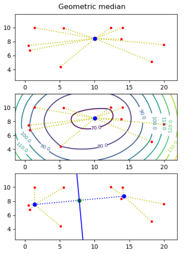
Motivation: Assume you want to build a drone tower from where to deliver parcels to costumers, and you know the destinations (points) where to deliver parcels. What is the optimal placement of the tower, if each drone can at most carry one parcel and needs to return to the tower between each delivery?
The geometric median of a point set S = { p1, ..., pn } in the plane is a point q (not necessarily a point in S), that minimizes the sum of distances to the points, i.e. minimizes ∑i=1..n |pi - q|, where |p - q| = ((px - qx)2 + (py - qy)2)0.5.
-
Create a function geometric_median that given a list
of points computes the geometric median of the point set.
Hint. Use the minimize function from the module scipy.optimize. - Make representative visualizations that show both the input point sets and the computed geometric medians. Examples should include point sets with two and three points, and a random point set.
- Use the matplotlib plotting function contour to plot a contour map to illustrate that it is the correct minimum that mas been found (the z-value for a point (x, y) in the contour map is the sum of the distances from (x, y) to all input points).
Next we want to find two points q1 and q2 such that the perpendicular bisector of q1 and q2 partitions the point set into the points closest to q1 and those closest to q2. We want to find two points q1 and q2 such that the sum of distances to the nearest point of q1 and q2 is minimized, i.e. ∑i=1..n min(|pi - q1|, |pi - q2|) is minimized.
To solve this problem one essentially has to consider all possible bisection lines, and to find the geometric median on both sides of the bisector, e.g. using the algorithm from question a). Assuming no three points are on a line, it is sufficient to consider all n(n-1)/2 bisector lines that go through two input points, and for each bisector line to consider the two cases where the two points on the line both are considered to be to the left or to the right of the line.
- Create a function two_geometric_medians that give a list of points p1, ..., pn computes two points q1 and q2 minimizing ∑i=1..n min(|pi - q1|, |pi - q2|). It can be assumed that no three points are on a line.
- Visualize your solution, showing imput points, q1 and q2, and the perpendicular bisector between q1 and q2.
- [optional] Extend your solution to handle the case where three or more points can be on a line. E.g. what is your solution if you have four points on a line?
Project II - Portfolio optimization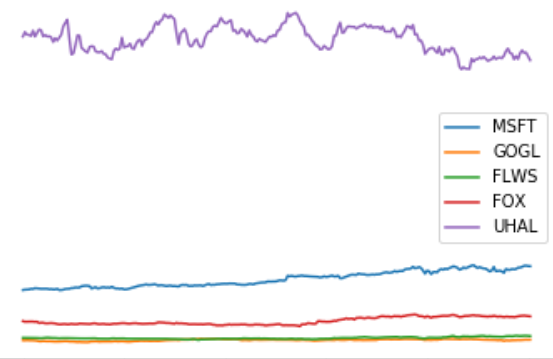
We consider the problem of choosing a long term stock portfolio, given a set of stocks and their price over some period under risk aversion parameter γ > 0.
Assume there are m stocks to be considered. The portfolio will be represented by a vector w ∈ ℝm, such that ∑i=1..m wi = 1. If wi > 0, you use a fraction wi of your total money to buy the i'th stock, while wi < 0 represent shorting that stock. In both cases we assume the stock is bought/shorted for the entire period.
Let pj,i represent the price of the i'th stock at time step j. If there are n time steps, then p ∈ ℝn×m is a matrix.
Let rj,i represent the fractional reward of stock i at time step j, i.e. rj,i = (pj,i - pj-1,i) / pj-1,i for j > 1.
We make the (unrealistic) assumption that we can model r by a random variable, distributed as a multivariate Gaussian, with estimated means
μ = E[r] ≃ 1/n · ∑j=1..n rj
and estimated variances
Σ = E[(r - μ)(r - μ)T] ≃ 1/n · ∑j=1..n [(rj - μ)(rj - μ)T]
Note that μi and Σi are the estimated mean and variance for stock i.
The distribution of returns using some w is then
Rw = N(μw, σw2)
μw = wTμ
σw2 = wTΣw
Now, we want to maximize for a balance between high return μw and low risk σw2. This leads to the following optimization problem, where we ant to find the value w* of w maximizing the following expresion:
maximize wTμ - γwTΣw
subject to ∑i=1..m wi = 1
where γ controls the balance between risk and return. A high value of γ indicate we are willing to take low risk and vise versa.
In this project you should find w* for different values of γ and using real stock values of your choice. The project consists of the following three questions.
- We need a module for collecting stock values. For this you can use the module pandas-datareader. Using this you should write a function get_prices([stock1, ..., stockk], step_size, period, exchange), that returns a tuple (stocks, p), where p[j, i] represents the opening price of stock i at time step j and stocks[i] is the name of the i'th stock (adjust the arguments to get_prices to the data available at your data source). Make a plot of p, where each stock is labeled with its name, e.g. MSFT or GOGL. You should use at least five stocks.
-
Calculate r, μ and Σ using the formulas above and
the p calculated in question (a). Plot
the probability density function (pdf) of the return of each
stock.
Hint. The method norm.pdf from the module scipy.stats might become convenient. -
Solve the optimization problem defined above for different values
of gamma, e.g. gammas = (np.arange(10) / 5) + 1, and plot
the pdf of each solution to a single plot with appropriate
legends. Finally create a scatter plot of how w* changes as
γ changes: For each value of γ plot the fraction of
each stock in the portfolio.
Project III - Simulations of NMR spectra of proteins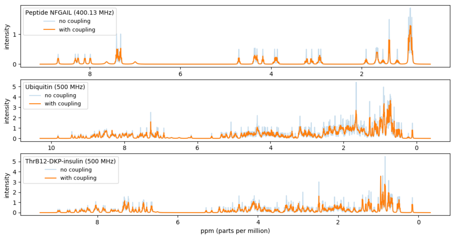
A fingerprint of a protein can be obtained by a nuclear magnetic resonance (NMR) experiment with a given spectrometer frequency (inputMHz). The fingerprint will be a spectrum of intensities over the frequency range. In this project you should compute a simulated approximation of the NMR fingerprint of a protein. In particular you should try to reproduce Figure 5(b) in [1]. The approximate fingerprint of a protein should be computed based on data available for the chemical shifts of the H-atoms in the protein and coupling data for H-atoms inside amino acids. We will approximate the spectrum with the sum of a set of Lorentz lines.
Protein molecules consist of one or more chains of amino acid residues. In the mandatory part of this project we will only consider proteins with one chain. Each amino acid in such a chain is identified by a a unique Seq_ID, an integer starting with one for the first amino acid in the sequence. The amino type is identified by Comp_ID (three letter abbreviation). Each atom in an amino acid has again a unique Atom_ID, where the first character is the atom type (i.e. in this project always H).
This project consists of the below tasks. Please remember to split your code into logical units, e.g. by introducing functions for various (recurring) subtasks.
- Download the files NFGAIL.csv, couplings.csv and 68_ubiquitin.csv.
-
The simplest Lorentz line is the function
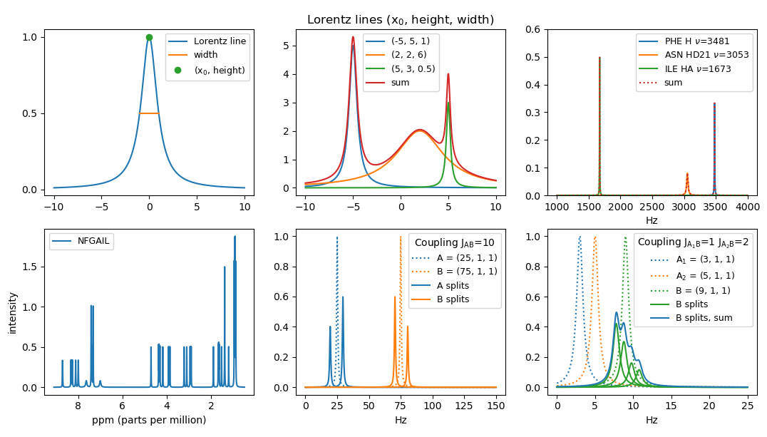
L(x) = 1 / (1 + x2) . Make a function Lorentz that given x returns L(x), where x can be either an integer, a float or a Numpy array. In the case of a Numpy array the function should be computed pointwise for each value. Plot the function for x ∈ [−10, 10] using matplotlib.pyplot (Hint: use numpy.linspace).
The function L has a maximum in (0, 1). We let (x0, height) denote the coordinates of the maximum of a Lorentz line. We let the width of a Lorentz line be the width of the peak at height height / 2, sometimes denoted full width half height (FWHH). The function L has width 2.
Note that the area below L is π = ∫(−∞,+∞) L(x) dx. -
Generalize your function Lorentz to take (optional keyword) arguments for
x0, height and width.
The resulting function should compute
Lx0, height, width(x) = height / (1 + (2 · (x − x0) / width)2) . Plot three Lorentz lines for the parameters (x0, height, width) being (-5, 5, 1), (2, 2, 6), and (5, 3, 0.5) for x ∈ [-10,10]. Plot also the sum of the three curves. Note that the area below a general Lorentz line is π · height · width / 2. - Our basic assumption is that each atom in a molecule contributes approximately one Lorentz line to the spectra. We will not use the same Lorentz parameters for all atoms. The width will e.g. depend on the atom_id and possibly also on the amino acid the atom is part of. Make a function peak_width(amino, atom_id) that returns the width for an atom in a specic amino acide and having a specific atom_id. If atom_id is H the width is 6. If (amino, atom_id) is one of the following four pairs (ASN, HD21), (ASN, HD22), (GLN, HE21), (GLN, HE22) the width is 25. For all other atom_id's the width is 4.
- We will denote a Lorentz line a peak and identify it by the triple (x0, height, width). For an atom (amino, atom_id) with assigned chemical shift value x0 (in Hz) we create a peak with width determined by peak_width and maximum value at (x0, height), where height is chosen such that the area below the Lorentz line is π. Create a function atom_peak(amino, atom_id, Hz) that returns the triple for the corresponding peak, where x0 = Hz = the chemical shift in Hz. Plot the peaks for the three atoms and assigned chemical shifts (PHE, H, 3481 Hz), (ASN, HD21, 3053 Hz), and (ILE, HA, 1673 Hz). Furthermore plot the sum of the three peaks.
- Create a function read_molecule that reads a list of atoms for a single protein from a CSV-file, where each row stores the description of an atom in the protein (most of the columns will not be used in this project). You can e.g. store each atom as a dictionary mapping column names to row values (Hint: use zip) or read the file as a pandas data frame.
- Read in the molecule description of the NFGAIL protein from the file NFGAIL.csv. For each of the 44 H-atoms create a peak assuming inputMHz = 400.13 MHz. The relevant columns are Atom_ID, Comp_ID (= amino acid), and Val. The column Val is the chemical shift in ppm, parts per million, but this value should be converted to Hz for calculations. To get the shift in Hz, multiply the Val value by inputMHz. Plot the sum of the peaks. Make the unit of the x-axis ppm (= Hz / inputMHz) and make the x-axis be decreasing from left to right.
-
To get a more refined spectrum we will take couplings between atoms into account.
Between two H-atoms A and B in an amino acid
(i.e. two peaks) there can be a coupling with
magnitude JAB, in the following just
denoted J, that influences the resulting spectrum. (Many
other factors influence the spectrum, but we will happily
ignore these in our simulations). The coupling between A
and B causes both peaks to be split into two new peaks
Ainner,
Aouter,
Binner and
Bouter,
where
Binner is closer to A than B,
and Bouter is further away from A than B.
In the following we only consider Binner
and Bouter (A is handled symmetrically).
The height of Bouter is smaller than the height of Binner,
the sum of their heights equals the height of B,
and their width equals the width of B.
Assume A and B have their maximum at
x0 = νA
and x0 = νB, respectively.
Let
Q = sqrt((νA − νB)2 + J2) The points Binner and Bouter are given by
νm = (νA + νB) / 2
σ = 1 if νA < νB, −1 otherwise
αinner = (1 + J / Q) / 2
αouter = (1 − J / Q) / 2 .νBinner = νm + σ · (Q − J) / 2 , heightBinner = heightB · αinner , widthBinner = widthB , Make a function apply_coupling(A, B, J) that takes two peaks A and B and computes the effect of A on B, when the coupling has magnitude J. Returns the list of the two peaks Binner and Bouter that B is split into. If J = 0 or x0(A) = x0(B), then only [B] is returned. Plot the four peaks resulting from the mutual coupling of two peaks A = (25, 1, 1) and B = (75, 1, 1) with J = 10.
νBouter = νm + σ · (Q + J) / 2 , heightBouter = heightB · αouter , widthBouter = widthB .
-
If an atom has couplings with several atoms the computations become slightly more involved. Assume B has couplings with k
atoms A1, A2, ..., Ak
with magnitudes
J1, J2, ..., Jk, respectively. In general the peak for B will be split into
2k peaks.
The basic idea is to start with the peak B.
Applying the coupling of B and A1 with magnitude J1 on B
results in a list L1 with at most two peaks.
Applying the coupling of B and A2 with magnitude J2 on each B' ∈ L1
results in the list L2 with at most four peaks. Applying A3 on the peaks in L2
results in eight peaks L3, etc.
Applying the coupling between Ai and B with magnitude J on a peak B' ∈ Li − 1 is done as applying A on B, except that the final computation of the points B'inner and B'outer are given byνB'inner = νB' − νB + νm + σ · (Q − J) / 2 , heightB'inner = heightB' · αinner , widthB'inner = widthB Extend your function apply_coupling to also be able to take a peak B' as an additional (optional) fourth argument. Note that for B' = B the function should return the same value as without the B' argument. Make a function apply_couplings([(A1, J1), (A2, J2), ..., (Ak, Jk)], B) to apply all couplings on B. Plot the four peaks and their sum resulting from applying A1 = (3, 1, 1) and A2 = (5, 1, 1) on B1 = (9, 1, 1) with magnitude J1 = 1 and J2 = 2, respectively. Note that permuting the list of (Ai, Ji)s should result in the same set of peaks for B.
νB'outer = νB' − νB + νm + σ · (Q + J) / 2 , heightB'outer = heightB' · αouter , widthB'outer = widthB
- Make a function to read the file couplings.csv that for each of the 20 amino acids contains the coupling magnitudes among the H-atoms inside the amino acid.
- Make a function split_comps that splits a list of atoms for a protein into a list of sublists, one sublist for each amino acid on the chain, i.e. split the list into sublists based on Seq_ID.
- Make a function comp_peaks(comp, couplings, input_MHz) that computes the peaks for all atoms in a amino acid (comp) by taking the table of couplings (from couplings.csv) into acount.
- Make a function protein_peaks(atoms, couplings, input_MHz) that takes a list of atoms for a protein, a table of couplings, and a frequency inputMHz and returns the resulting peaks by applying all couplings. Apply the function to the data from NFGAIL.csv with inputMHz = 400.13 MHz. Plot the sum of the resulting 542 peaks. Make the unit of the x-axis ppm (= Hz / inputMHz) and make the x-axis be decreasing from left to right. Your result should be a reproduction of 5(b) in [1].
| Protein | Uncoupled peaks | Coupled peaks |
|---|---|---|
| NFGAIL | 44 | 542 |
| Ubiquitin | 556 | 6805 |
| ThrB12-DKP-insulin | 329 | 3338 |
The following tasks are optional.
In the previous tasks you were given CSV-files with the description of proteins only containing one chain. The following tasks ask you to download protein descriptions from the Biological Magnetic Resonance Data Bank (BMRB, bmrb.wisc.edu) containing an arbitrary number of chains. In the data bank each data set for a molecule has a unique Entry_ID value. Each chain is identified by a unique Entity_ID. Each amino acid in a chain has a unique Seq_ID (and amino type Comp_ID) and each atom in an amino acid has again a unique Atom_ID.
- Download the file Atom_chem_shift.csv (700+ MB) from www.bmrb.wisc.edu > Bulk access > CSV relational data tables. This file contains the atom shift data for all data sets on the web site.
- Write a function csv_extract that given a value Entry_ID, from Atom_chem_shift.csv extracts all rows with value Entry_ID in column Entry_ID and outputs the resulting rows to a new CSV-file. Test this with Entry_ID = 68 and Entry_ID = 6203. The result for Entry_ID = 68 should be the 556 atoms as provided in the file 68_ubiquitin.csv (but with additional columns). The result for Entry_ID = 6203 should be a file with a header row plus 329 data rows (atoms) for ThrB12-DKP-insulin. (Hint: Avoid reading the whole table into memory. If you e.g. read the complete table using Pandas, the data will take up memory ≈ 3 × file size. Instead scan through the file using the csv module and only have the current line in memory. Scanning through the 700+ MB should be possible within in the order of a minute.)
- Update the function split_comps to be able to handle more than one chain of amino acids. In particular each comp should now be identified not only by Seq_ID but by the pair (Entity_ID, Seq_id).
- Extract data for ThrB12-DKP-insulin (Entry_ID = 6203) from Atom_chem_shift.csv and plot the resulting simulated spectrum for inputMHz = 500 MHz. Note that the data for ThrB12-DKP-insulin consists of two chains of 131 and 198 atoms, respectively. You can find the Entry_ID value for your favorite protein by searching the BMRB data base at www.bmrb.wisc.edu.
References
[1] Fast simulations of multidimensional NMR spectra of proteins and peptides. Thomas Vosegaard. Magnetic Resonance in Chemistry. 56(6), 438-448, 2018. DOI: 10.1002/mrc.4663.
Project IV - MNIST Image Classification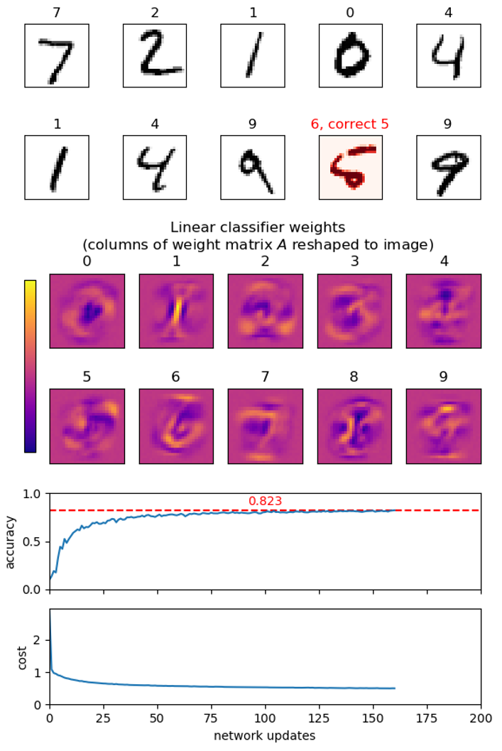
In this project we are going to create a very simple neural network (linear classifier) to identify the handwritten digits from the MNIST database - often considered the "Hello World" problem in neural networks. In this problem we are given grayscale images of size 28 × 28 showing handwritten digits and are going to classify them into the 10 classes 0 - 9, depending on the digit depicted in the image. The MNIST database consists of 60.000 images to train your network on and 10.000 images to test the quality (accuracy) of the resulting network. For all images the correct label 0 - 9 is part of the database. There exist many of-the-shelf modules for this problem in Python, e.g. Keras, TensorFlow, scikit, and PyTorch, but in this project we are going to build a solution using pure Python from scratch.
A good introduction to the topic are the following four videos from the YouTube channel by 3BLUE1BROWN: Neural Network (19:13), Gradient Descend (21:00), Backpropagation (13:53), and Backpropagation Calculus (10:17). The few mathematical equations required in this project for performing simple backpropagation are stated explicitly below.
You are not allowed to use NumPy, Keras, etc. in the questions below (if not stated otherwise).
The first group of tasks concerns reading the raw data and visualizing them.
-
From
yann.lecun.com/exdb/mnist/
download the following four files:
- t10k-images.idx3-ubyte.gz (1.6 MB)
- t10k-labels.idx1-ubyte.gz (4.4 KB)
- train-images.idx3-ubyte.gz (9.6 MB)
- train-labels.idx1-ubyte.gz (28.3 KB)
-
Make a function read_labels(filename) to read a file
containing labels (integers 0-9) in the format described under
"FILE
FORMATS FOR THE MNIST DATABASE". The function should return
a list of integers. Test your method on the
files t10k-labels.idx1-ubyte.gz and train-labels.idx1-ubyte.gz (the
first five values of the 10.000 values in t10k-labels.idx1-ubyte.gz are
[7, 2, 1, 0, 4]).
The function should check if the magic number of the file is 2049.
Hint: Open the files for reading in binary mode by providing open with the argument 'rb'. You can either uncompress the files using a program like 7zip, or work directly with the compressed files using the gzip module in Python. In particular gzip.open will be relevant. To convert 4 bytes to an integer int.from_bytes might become useful. - Make a function read_images(filename) to read a file containing MNIST images in the format described under "FILE FORMATS FOR THE MNIST DATABASE". Test your method on the files t10k-images.idx3-ubyte.gz and train-images.idx3-ubyte.gz. The function should return a three dimensional list of integers, such that images[image][row][column] is a pixel value (an integer in the range 0..255), and 0 ≤ row, column < 28 and 0 ≤ image < 10000 for t10k-images.idx3-ubyte.gz. The function should check if the magic number of the file is 2051.
- Make a function plot_images(images, labels) to show a set of images and their corresponding labels as titles using imshow from matplotlib.pyplot. Show the first few images from t10k-images.idx3-ubyte.gz with their labels from t10k-labels.idx1-ubyte.gz as titles. Remember to select an appropriate colormap for imshow.
A linear classifier consists of a pair (A, b), where A is a weight matrix of size 784 × 10 and b is a bias vector of length 10. An image containing 28 × 28 pixels is viewed as a vector x of length 784 (= 28 * 28), where the pixel values are scaled to be floats in the range [0, 1]. In the following we denote this representation an image vector. The prediction by the classifier is computed as
a = xA + b,where a = (a0, ..., a9), i.e. the result of the vector-matrix product xA, that results in a vector of length 10, followed by a vector-vector addition with b. The predicted class is the index i, such that ai is the largest entry in a.
In the follow we will apply the cost measure mean squared error to evalutate how close the output a = xA + b of a network (A, b) is for an input x to the correct answer y, where we assume that y is the categorical vector of length 10 for the correct label, i.e. yi = 1 if i = label, and 0 otherwise:
cost(a, y) = sumi ((ai − yi)2) / 10We use the mean squared error because is has an easy computable derivative, although better cost functions exist for this learning problem, e.g. softmax.
Below you will be asked to compute weights (A, b) using back propagation. To get started, a set of weights (A, b) is available as mnist_linear.weights. The weights were generated using the short program mnist_keras_linear.py using the neural networks API Keras running on top of Google's TensorFlow. The network achieves around 92% accuracy on the MNIST test set (you should not expect to reach this level, since this network is trained using the softmax cost function).
- Optional: You should be able to reproduce a similar weight file (but not exactly the same) by runing the script, after pip installing Keras. This is not part of the project. Currently TensorFlow is not supported for Python 3.8, so you need to install Python 3.7 to run the script.
The second group of tasks is to load and save existing linear classifier networks and to evaluate their performance, together with various helper functions. In the following we assume the vector b to be represented by a standard Python list of floats and the matrix A to be represented by a list-of-lists of floats.
- Write functions linear_load(file_name) and linear_save(file_name, network) to load and save a linear classifier network = (A, b) using JSON. Test your functions on mnist_linear.weights .
- Write function image_to_vector(image) that converts an image (list-of-lists) with integer pixel values in the range [0, 255] to an image vector (list) with pixel values being floats in the range [0, 1].
- Write functions for basic linear algebra add(U, V), sub(U, V), scalar_multiplication(scalar, V) multiply(V, M), transpose(M) where V and U are vectors and M is a matrix. Include assertions to check if the dimensions of the arguments to add and multiply fit.
-
Write a function mean_square_error(U, V) to compute the
mean squared error between two vectors.
Examples: mean_square_error([1,2,3,4], [3,1,3,2]) shoule return 2.25. - Write function a function argmax(V) that returns an index into the list V with maximal value (corresponding to numpy.argmax). E.g. argmax([6, 2, 7, 10, 5]) should return 3.
-
Implement a function categorical(label, classes=10) that
takes a label from [0, 9] and returns a vector of
length classes, with all entries being zero, except entry
label that equals one. For an image with this label, the
categorical vector is the expected ideal output of a perfect
network for the image.
Example: categorical(3) should return [0,0,0,1,0,0,0,0,0,0]. - Write a function predict(network, image) that returns xA + b, given a network (A, b) and an image vector.
-
Create a function evaluate(network, images, labels) that
given a list of image vectors and corresponding labels, returns
the tuple (predictions, cost, accuracy),
where predictions is a list of the predicted labels for the
images, cost is the average of mean square errors over all
input-output pairs, and accuracy the fraction of inputs
where the predicted labels are correct. Apply this to the loaded
network and the 10.000 test images in t10k-images. The accuracy
should be around 92%, whereas the cost should be 222 (the cost is very
bad since the network was trained to optimze the cost measure softmax).
Hint. Use your argmax function to convert network output into a label prediction. - Extend plot_images to take an optional argument prediction that is a list of predicted labels for the images, and visualizes if the prediction is correct or wrong. Test it on a set of images from t10k-images and their correct labels from t10k-labels.
- Column i of matrix A contains the (positive or negative) weight of each input pixel for class i, i.e. the contribution of the pixels towards the image showing the digit i. Use imshow to visualize each column (each column is a vector of length 784 that should be reshaped to an image of size 28 × 28).
The third group of tasks is to train your own linear classifier network, i.e. to compute a matrix A and a vector b.
-
Create function create_batches(values, batch_size) that
partitions a list of values into batches of size batch_size,
except for the last batch, that can be smaller. The list should be
permuted before being cut into batches.
Example: create_batches(list(range(7)), 3) should return [[3, 0, 1], [2, 5, 4], [6]]. -
Create a function update(network, images, labels) that
updates the network network = (A, b) given
a batch of n image vectors and corresponding output labels
(performs one step of a stochastical gradient descend in the
784 * 10 + 10 = 7850 dimensional space where all entries of A
and b are considered to be variables).
For each input in the batch, we consider the tuple (x, a, y), where x is the image vector, a = xA + b the current network's output on input x, and y the corresponding categorical vector for the label. The biases b and weights A are updated as follows:bj −= σ · (1 / n) · ∑(x,a,y) 2 · (aj − yj) / 10
For this problem an appropriate value for the step size σ of the gradient descend is σ = 0.1.
Aij −= σ · (1 / n) · ∑(x,a,y) xi · 2 · (aj − yj) / 10
In the above equations 2 · (aj −yj) / 10 is the derivative of the cost function (mean squared error) wrt. to the output aj, whereas xi · 2 · (aj − yj) / 10 is the derivative of the cost function w.r.t. to Aij — both for a specific image (x, a, y). -
Create a function learn(images, labels, epochs,
batch_size) to train an initially random network on a set of
image vectors and labels.
First initialize the network to contain random weights: each value
of b to be a uniform random value in [0, 1], and each
value in A to be a uniform random value in [0, 1 / 784]. Then
perform epochs epochs, each epoch consiting of
partitioning the input into batches of batch_size
images, and calling update with each of the batches.
Try running your learning function with epochs=5
and batch_size=100 on the MNIST training set
train-images and train-labels.
Hint. The above computation can take a long time, so print regularly a status of the current progress of the network learning, e.g. by evaluating the network on (a subset of) the test images t10k-images. Regularly save the best network seen so far.
Here are some additional optional tasks. Feel free to come up with your own (other networks, other optimization strategies, other loss functions, ...).
-
Optional. Instead of using the mean squared error as the
cost function try to use the categorical cross entropy (see e.g. this blog): On
output a where the expected output is the categorical
vector y, the categorical cross
entropy is defined as CE(y, softmax(a)),
where softmax(a)i =
eai
/ (∑j eaj)
and the cross entropy is defined as
CE(y, â) = − ∑i
(yi · log âi).
In update the derivative of the cost function
w.r.t. output aj should be replaced by
eaj
/(∑k eak)
− yj.
Note. softmax(a) is a vector with the same length as a with values having the same relative order as in a, but elements are scalled so that softmax(a)i ∈ ]0,1[ and 1 = ∑i softmax(a)i. Furthermore, since y is categorical with yi = 1 for exactly one i, CE(y, softmax(a)) = log(∑j eaj) − ai. -
Optional. Visualize the changing weights, cost, and accuracy during the learning.
Hint. You can use matplotlib.animation.FuncAnimation, and let the provided function apply one batch of training data to the network for each call. -
Optional: Redo the above exercises in Numpy. Create a generic
method for reading IDX files into NumPy arrays based on the
specification "THE IDX FILE FORMAT". Data can be read from a
file directly into a NumPy array using numpy.fromfile and
an appropriate
dtype.
Hint. np.argmax(test_images.reshape(10000, 28 * 28) @ A + b, axis=1) computes the predictions for all tests images, if they are all in one NumPy array with shape (10000, 28, 28). - Optional: Compare your pure Python solution with your Numpy implementation (if you did the above optional task) and/or the solution using Keras, e.g. on running time, accuracy achieved, epochs.
-
Optional: Try to take a picture of your own handwritten
letters and see if your program can classify your digits. It is
important that you preprocess your images to the same nomalized
format as the original MNIST data: Images should be 28 × 28
pixels where each pixel is represented by an 8-bit greyscale value
where 255 is black and 0 is white. The center of mass should be in
the center of the image. In the test data all images were first
scaled to fit in a 20 × 20 box, and then padded with eight
rows and columns with zeros to make the center of mass the center
of the image,
see yann.lecun.com/exdb/mnist.
Hint: PIL.Image.resize from the Pillow (Python Imaging Library) might be usefull. Remember to set the resampling filter to BILINEAR.
Project IV - Open topic
You can also define your own project. There are some aspects that needs to be addressed.
- Some minimal amount of Python 3 code must be produced.
- Use at least two different Python modules.
- Some data must be visualized, e.g using matplotlib, but any visualization module or domain specific library, like for chemistry, can be used.